Gaussianograph: Oakland Cemetery

Sep 30, 2026 · @Joel Silverman

Oakland Cemetery was founded in 1850 as Atlanta Cemetery, six acres of ground on the outskirts of a brand-new railroad town. As the city grew around it, the cemetery grew to 48 acres, and today about 70,000 people are buried there, from governors and mayors to Margaret Mitchell, Kenny Rogers, and golfing legend Bobby Jones, to thousands of unknown souls whose names have worn off their stones. When you walk through Oakland, you're reading the history of Atlanta off the headstones, but it gets harder to read every year. Marble dissolves slowly in the rain and the people who remembered whose name was carved on a broken tablet are eventually gone themselves. Historic preservation starts with a record of what is there, and for a massive burial ground as old as Oakland, a complete record has been out of reach.

For most of the last twenty years the tool for turning photographs into a 3D model has been photogrammetry, which matches points across overlapping pictures and builds a mesh surface out of them. It works well on a building or a statue. But across a whole landscape it breaks down. Trees turn into melted lumps, fences and branches disappear, and tens of thousands of high-resolution photographs overwhelm both the software and the computer running it.

The unsatisfactory way Oakland's trees are rendered by Google Earth's old-school photogrammetry.

In December 2022, Historic Oakland Foundation and Emory University asked me to make a 3D scan of Oakland. I had spent time as an artist in residence with Emory's Data Visualization Lab, 3D scanning the coastline of Sapelo Island to document historic archaeological sites and measure how a shoreline moves as the climate changes. I flew the cemetery with a DJI Matrice 300 survey drone carrying a 45-megapixel camera, flying day-long missions at two different elevations and from every angle, and wound up at the end with 12,828 photographs and half a terabyte of data. With the reconstruction software of 2022, the set could not be modeled at all. I wasted weeks trying to make it work. I put the project on the shelf for a few years and waited for the technology to catch up.

It caught up with 3D Gaussian splatting, which builds a scene from millions of small, soft, colored shapes fitted to the photographs, each one able to hold a leaf, a patch of lichen or a shadow.

Left, one of my source photographs from the 300-foot flight. Right, a video rendered from a Gaussian Splat of the scene.

Over 2025 and 2026 gaussian splats made great leaps in realism, and training one became something a computer can largely do on its own. AI coding agents grew up at the same time: Claude Code can now stay with a single problem for weeks at a time. I set up a dedicated graphics workstation and designed software to cut the site into 35 tiles, train each one, and assemble them into a single world of 169,303,657 gaussians, detailed enough to fly through like a video game. It has none of the usual tells of early-gen gaussian splatting, with stray floaters hanging in the air:

A gaussian splat with typical "floaters."

I used Unreal Engine to render the model into cinematic shots, which is the same way Hollywood's virtual production works. Star Wars' The Mandalorian pioneered this approach in 2019, when Industrial Light & Magic surrounded actors with a curved wall of LED screens, called "The Volume", showing immersive but fake digital sets rendered live in Unreal Engine.

The Volume on the set of The Mandalorian. From Industrial Light & Magic's The Virtual Production of The Mandalorian Season One.

The tools built for big-budget television are now within reach of a solo artist or historian, and they let an audience step inside a place, or a reconstruction of its past, and look around.

What a gaussian splat is

A splat model is built backwards from photographs. The software scatters millions of small translucent blobs through space, each with a position, a shape, an opacity and a color that shifts slightly with the viewing angle. Then it renders the blobs from the spot where each photograph was taken, compares them, and nudges every blob to close the gaps, thousands of times over, until they resolve into, say, a granite obelisk, the bark of an magnolia tree, or a well-worn brick path.

Photogrammetry builds a 3D topography and paints the photographs onto it as textures, on the surface like the hard candy shell of chocolate on a DQ soft serve ice cream, which is why its trees come out so weird looking. A splat has no shell, so leaves, railings and grass can be as fine as the photographs allow.

How the model was made

Oakland's vast expanse of detail was too large for any computer to generate a model all in one pass. I did it in sections, first laying a grid of 36 squares over it, like the sheets of an old Sanborn fire-insurance atlas, and "trained" the model in 36 pieces, each section looking only at the photographs taken when I flew over that area. Since each square took two to three hours on a graphics card, this took my computer busy for almost a week. I finally did something I should have done years ago, and set up the graphics workstation in my studio onto a network so I could stay off that computer while it worked and just monitor it from my everyday work laptop without needing to even go to my studio.

Then the squares had to get fused into one scene. I cut off any overlaps so that it fit together like a tidy jigsaw puzzle, and cleaned up the floaters, haze and glare the software had made during the training. I drew the outer edge by hand along the far curb of the streets around the cemetery, so the cemetery sits on its own block that can be dropped into a larger digital twin of the neighborhood (say, in Cesium or Google Earth.) Half-scanned ghosts of structures outside the scanning radius occur during any gaussian training, and these had to be cut out, except I kept the facade of the Fulton Bag and Cotton Mills across the railroad tracks, because I love that building and it's an iconic view familiar to visitors inside the cemetery. Wherever my low 125' flight had missed a patch of ground (say from a tree branch obstruction), I filled it with detail from the higher flight pass.

The finished 3D world "lives" in Unreal Engine. To render a cinematic, I just need to fly a virtual camera through it the way I'd fly the drone, and render each shot one frame at a time. A companion model, lower in resolution, lives in Blender on my laptop, where it's easy to select flyover viewpoints to send to Unreal Engine for the cinematic renders. I don't really even know how to use Unreal Engine, but Claude Code does, and throughout this process I've been creating gorgeous cinematics without ever driving Unreal myself.

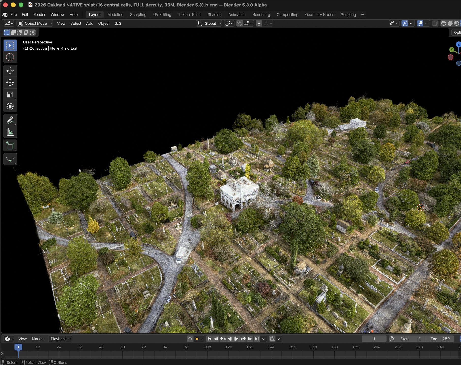
Making a 3D Gaussian Splat

I wrote this up in detail mostly so I can retrace my steps the next time someone asks me to make a large 3D reconstruction of a historic site, but also because I want to encourage people to try turning large drone-scanned site photo sets into 3D gaussian splat models for themselves. It's a complex workflow, but easier than it ever was before, that's for sure.

1. Capture

I flew a DJI Matrice 300 with a DJI Zenmuse P1 camera, the P1 is an SLR with interchangeable lenses, it shoots razor-sharp high-res 8K images. I shot the scene twice:

• A high oblique flight at 300 feet: 3,270 photographs in DJI's Smart Oblique mode, which tilts the camera through five angles at each stop, so it sees the sides of monuments, walls and trees.

• A low flight from 125 feet: This set was 3,319 photographs where each pixel represents just half a centimeter on the ground. This is almost, but not quite, detailed enough to actually read the text on most of the grave markers in the cemetery. I'm working on getting it even better because this level of detail at this scale would be the holy grail of large-site reconstruction. If you have advice for me, please reach out.

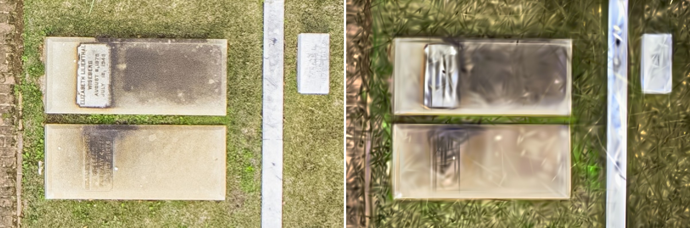
Left, a crop of a low-flight photograph, where the marker for Elizabeth Lilienthal Wiseberg (1875 to 1948) reads clearly. Right, the same grave marker seen in the model at the same magnification: the stones are in place and the letters are blurred.

Tilted views give tall things their shape; straight-down views make the ground sharp. So in the finished model, trees and monuments hold up from the side, but open ground smears when the camera skims across it. Plan your camera moves around that.

I needed to batch-color grade all the photographs to uniform brightness and color, since different angles of the model would show any color shift or difference in cloud cover between flights.

2. Align both flights as one

I aligned all 6,589 photographs together in RealityScan 2.2 (until recently, RealityScan was known as RealityCapture). I used to do this through the laborious RealityCapture workflow, but now Claude Code can do this part autonomously without much help, through a terminal CLI interface. They call running software this way "headless" because your computer monitor doesn't even need to be on, the AI agent is running the bare code of the software without even needing the visual interface.

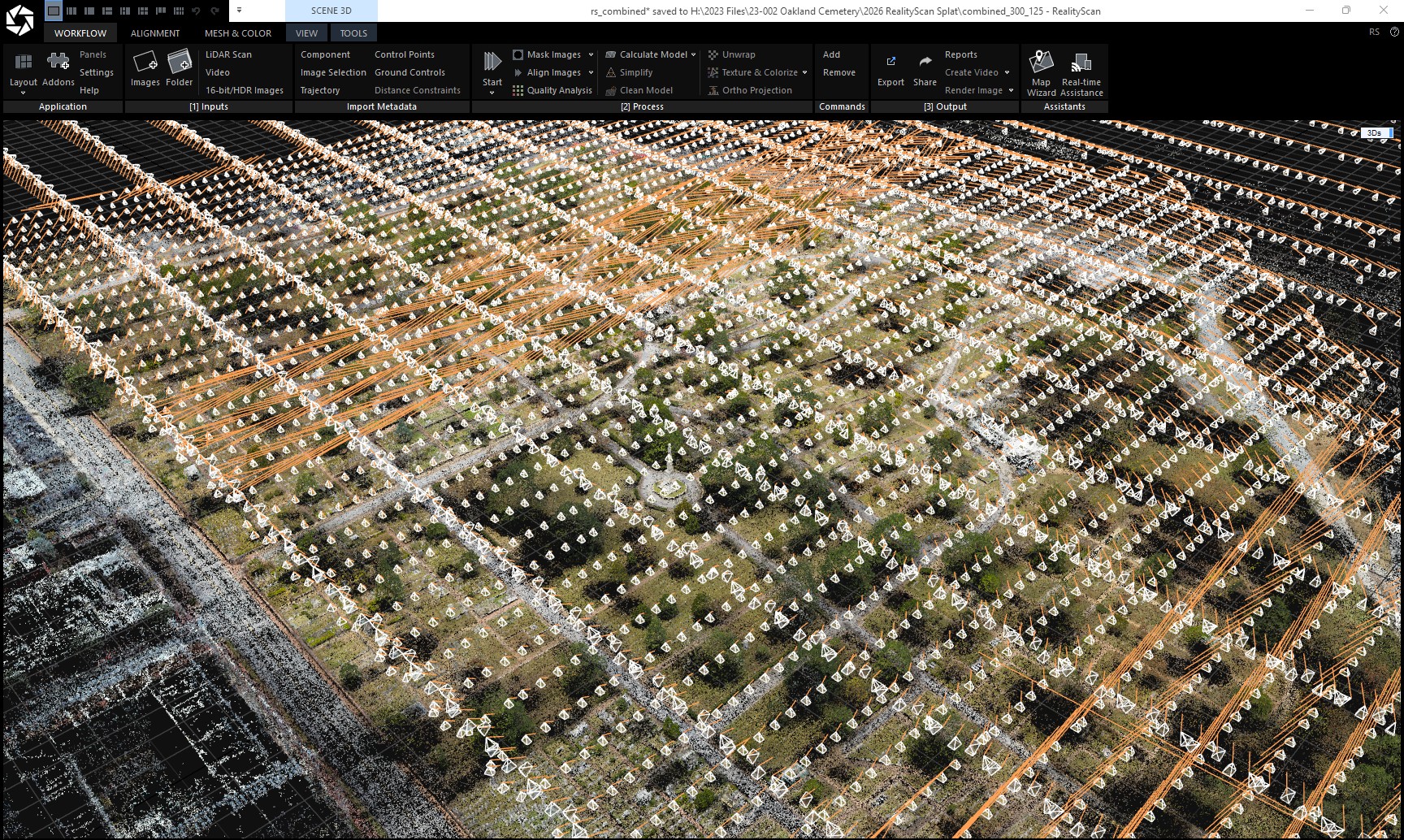
RealityScan's alignment map of this scene: each white pyramid represents one photograph's camera, hovering over the points it matched.

The result was 6,588 photographs mapped out in relationship to each other with millions of machine-vision detected control points. I exported it in COLMAP and figured out that aligning the two flights together led to a result better than any gaussian splat scene I'd ever seen before. This is something that RealityScan or the splat training softwares I've used like LichtFeld or Spirula can't do by themselves, combining the different perspectives of two altitudes was a crazy AI computational task that had Claude crunching away on my Nvidia 3090 graphics workstation for days to solve. (The 3090 was a best-in-class GPU five years ago when I bought it, I'm not sure if slightly more recent cards are any faster at insanely intensive tasks like this.) When you look at them in a side-by-side test, it's clear that the combined fusion of a 125 foot flight and a 300 foot flight was cleaner and more detailed than a model made from either flight alone.

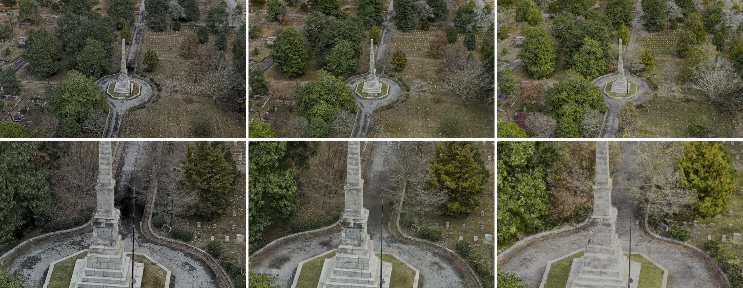
One camera position from the obelisk orbit, three models. Left, trained on the 300-foot flight only (51,584,891 gaussians for the site). Centre, trained on both flights (177,903,398). Right, trained on the 125-foot flight only, the version in the finished world (227,881,884 before the reduction to 73%). Below, the same patch at full resolution.

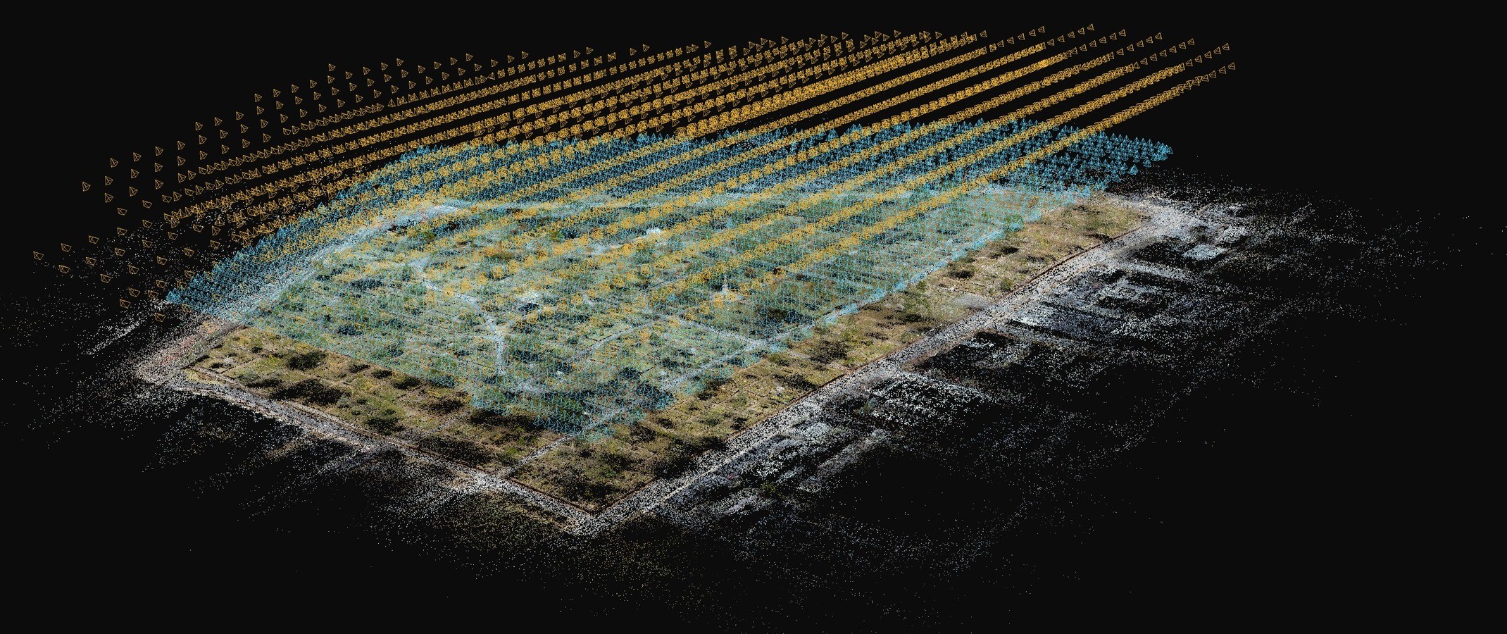
Every aligned camera position over the sparse point cloud: 3,270 from the 300-foot flight in gold and 3,318 from the 125-foot flight in blue.

3. Cut the site into tiles

No graphics card can train half a terabyte of photographs as one model, so I cut the giant site into a six-by-six grid. I got the idea from "open world" video games like Grand Theft Auto, where separate scenes are seamlessly stitched together and the player never knows it. Each square learns only from the photographs that look at it, plus a margin of about 20% past its edges that gets trimmed off afterwards, so neighboring squares meet without a seam. One corner square had been seen by only two photographs, so I dropped it and kept 35.

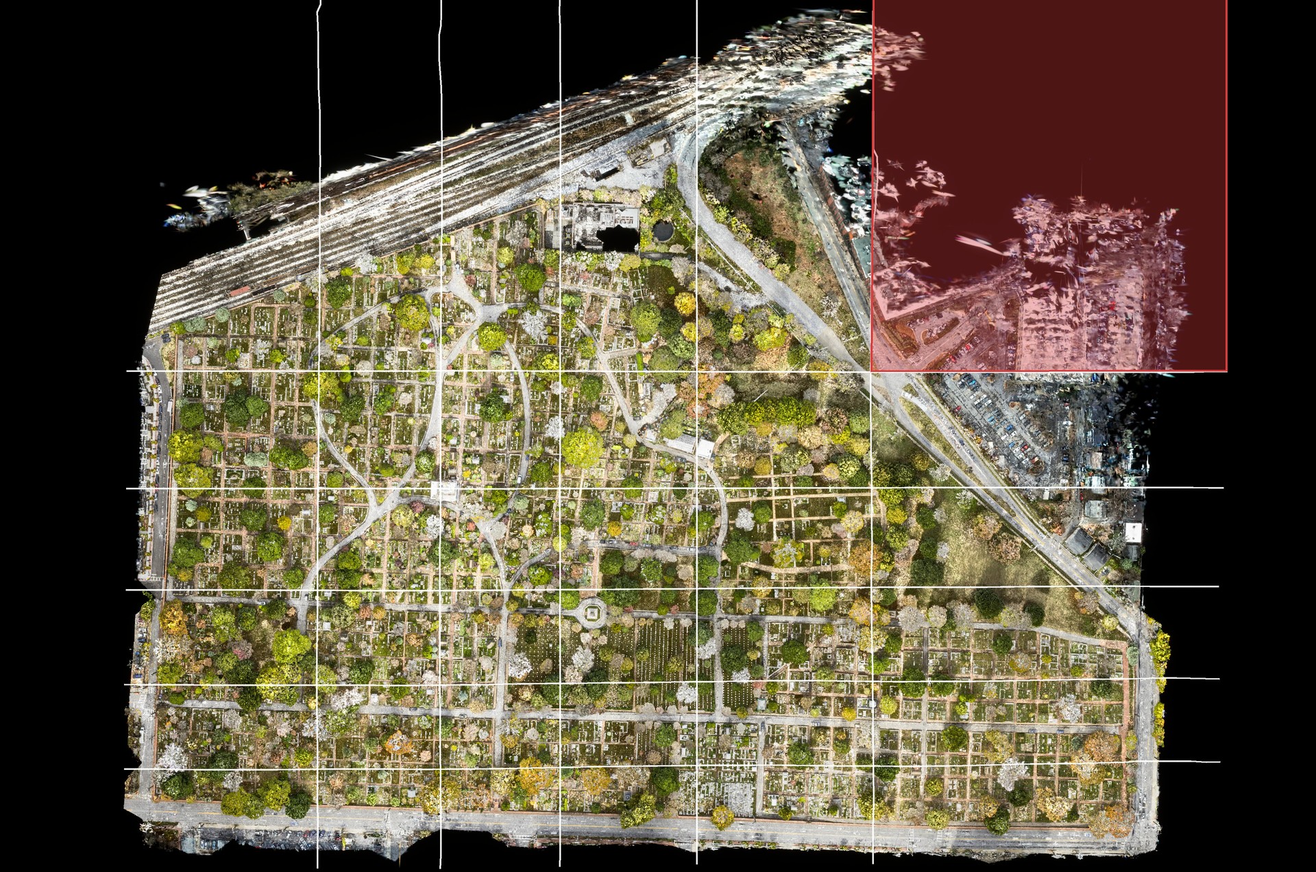
The six-by-six training grid over the finished world. The red square is the dropped corner; the mill fill patch now covers part of it.

4. Test before committing

Train two or three squares first and judge them by eye. I compared 12 million gaussians per square with 18 million and couldn't tell them apart, because the detail is limited by the photographs, so I wound up capping resolution of every square to "just" 12 million.

5. Train each tile

To train the model, I used the open source LichtFeld Studio (github.com/MrNeRF/LichtFeld-Studio) and an NVIDIA driver from the 570 series.

In plain terms: 20,000 training steps, at most 12 million gaussians, full-resolution photographs, and color that shifts with the viewing angle. Each square needs about 14 GB of graphics memory and took two to three hours on a 48 GB card, 80 to 110 card-hours for the whole site.

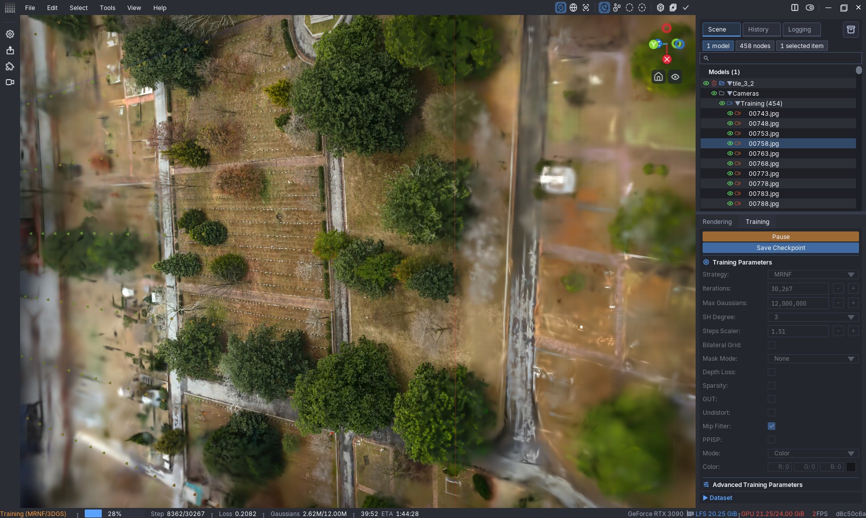
LichtFeld Studio in action, seen from one training camera out of 30,267 views used.

6. Clean each tile

Three passes, square by square. First, crop each square to its exact edges. Second, remove the giant see-through shapes the trainer invents to explain cloud shadows and glare, which read from above as burnt patches and white bloom: any gaussian whose smallest axis tops 0.5 meters or whose middle axis tops 0.75 meters. Third, remove junk floating above or sunk below the site: anything 30 meters over or 8 meters under the local ground, and sparse specks more than 8 meters up with fewer than 30 neighbors in a 6-meter cube. Together they removed 4,612,934 of 232,494,818 gaussians (1.98%).

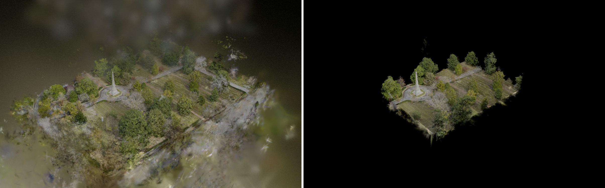
One square as trained (left), with its margin and haze, and the same square cropped and cleaned (right).

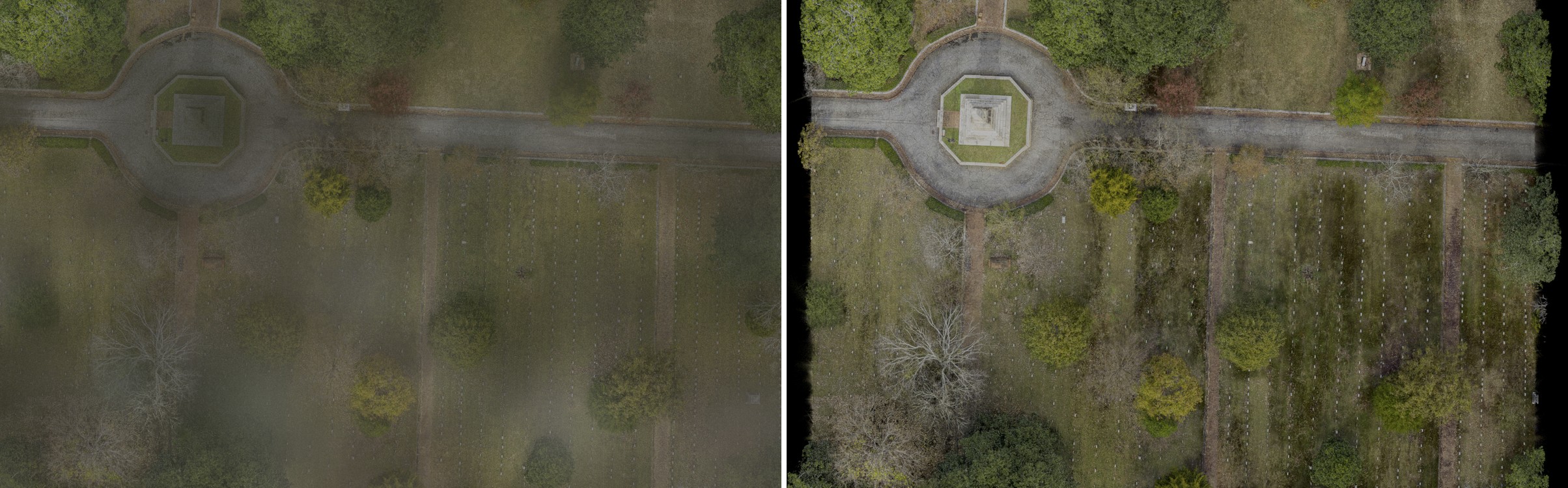
The same square from straight above: the haze the trainer invented (left) and the square after cleanup (right).

7. Draw the boundary and fill the holes

I traced the keep line by hand along the far curbs, cut out every building outside the walls using OpenStreetMap footprints, and added the mill back as its own keep area. Cut along the city's own seams, such as curbs, pavement edges and building faces, so the edge never looks like scissors through a lawn. Draw the line in the model's own coordinates; in the wrong frame it lands up to 21 meters off. The holes the low flight never covered were filled from the high flight, 3,188,924 gaussians in three patches.

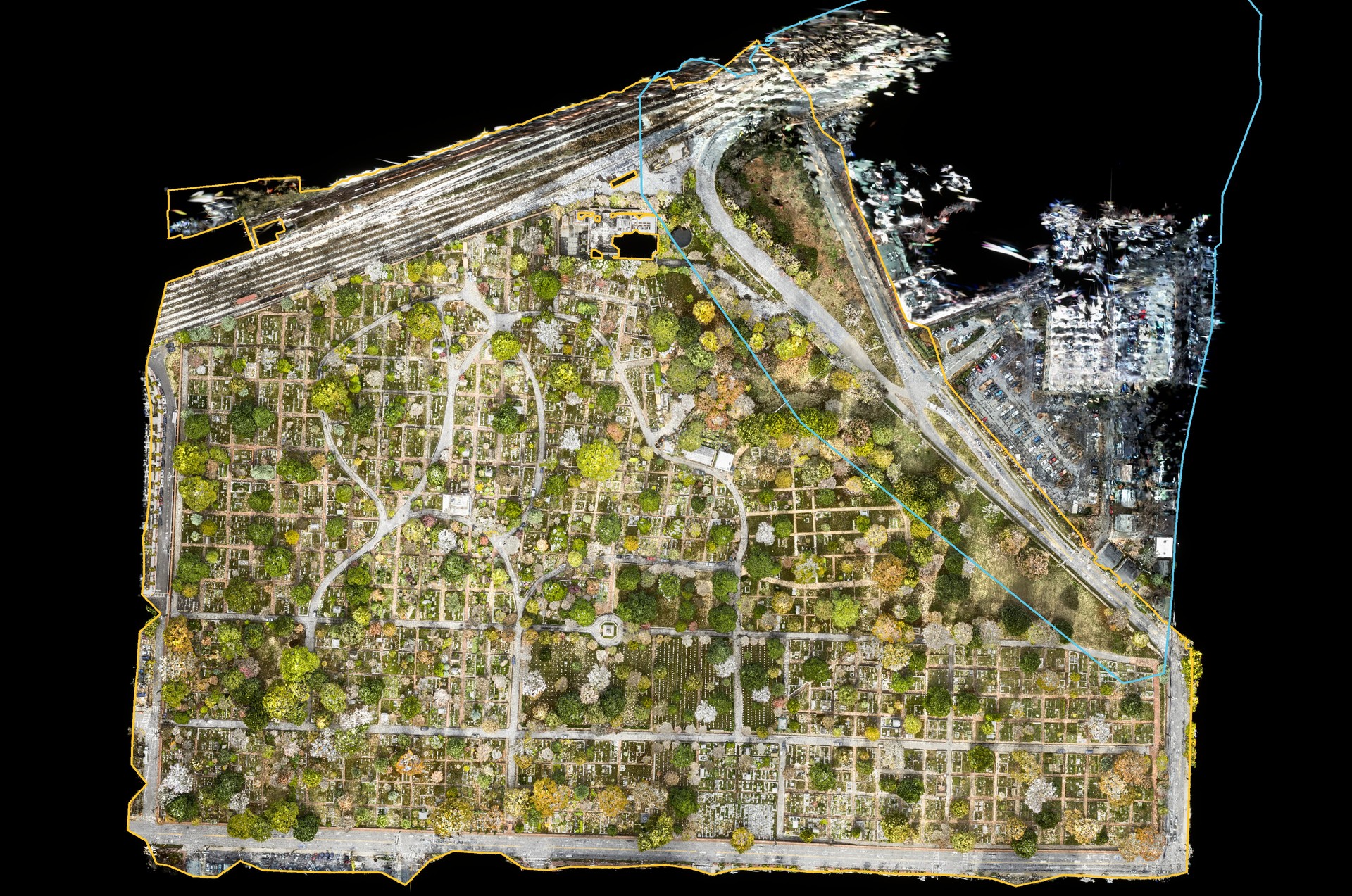
The keep line, traced by hand along the far curbs (gold), and the mill's separate keep area (blue).

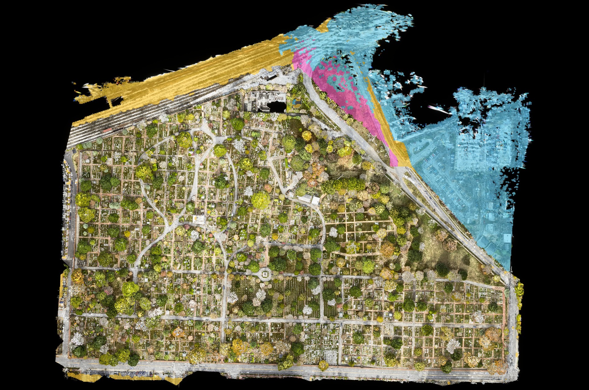
The three fill patches from the high flight: the northeast tree island (pink), the street margins (gold) and the mill (blue).

8. Fit the world to the card

Unreal needs about 136 bytes of memory per gaussian, so the full site, about 31.6 GB, won't fit on a 24 GB card. I reduced it to 73% of trained density, a figure I chose by eye. Don't thin at random, or surfaces go see-through. Keep the most important gaussians in each small volume and raise the survivors' opacity so the volume still blocks the same light: for a kept fraction p, opacity α becomes 1 − (1 − α)^(1/p), after converting the stored log-odds value to an opacity. Below a kept fraction of about a quarter, this breaks down.

9. A last pass for floaters

Even then, specks hung a few meters over some trees. The final pass breaks the world into quarter-meter cubes of visible gaussians (opacity 0.1 or more), in 50-meter tiles overlapping by 6 meters, and finds every piece that isn't connected to the rest. A piece goes only if it floats at least 1.5 meters clear, over ground, and outside the fill patches; anything closer is a real branch tip. At half-meter cubes the specks chain together and hide in the canopy. I checked every area from four sides and from above, before and after. The pass removed 234,455 gaussians in 4,952 pieces, leaving 169,303,657, written as a new numbered copy with every removed gaussian kept on file.

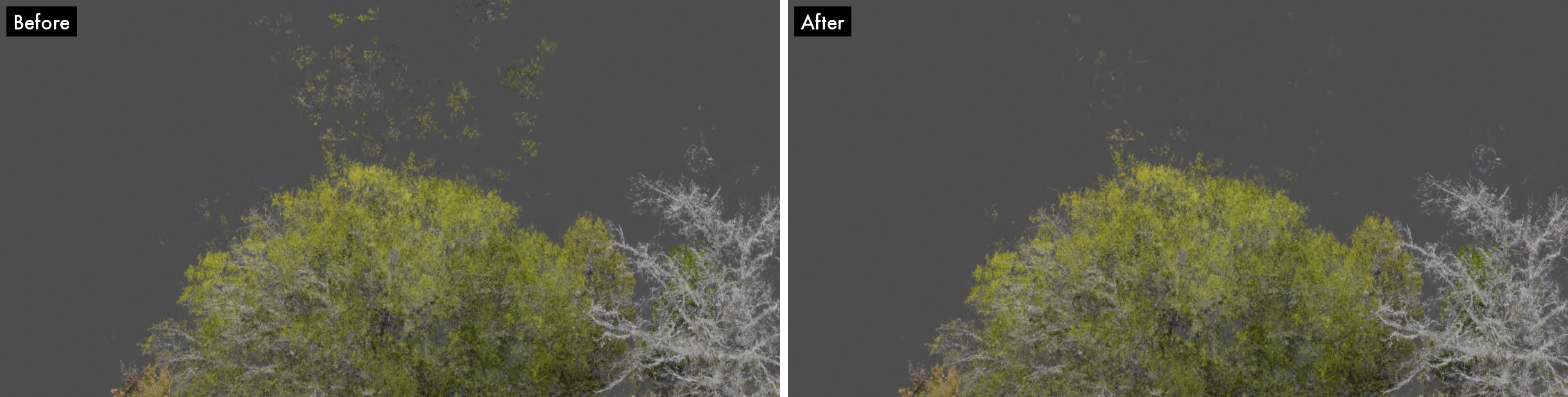
Floaters over a tree crown, seen from the side, before and after the last pass.

10. Render in Unreal

I render in Unreal Engine 5.8.1, built from source, with the free NanoGS splat plugin (github.com/TimChen1383/NanoGaussianSplatting). As shipped, the plugin rounds positions to 16 bits, about 16-centimeter steps this far from the origin, and sorts the scene in batches. Those two shortcuts make tile seams flash and dry ground shimmer like wet pavement, so I patched it to keep full precision and sort everything in view at once.

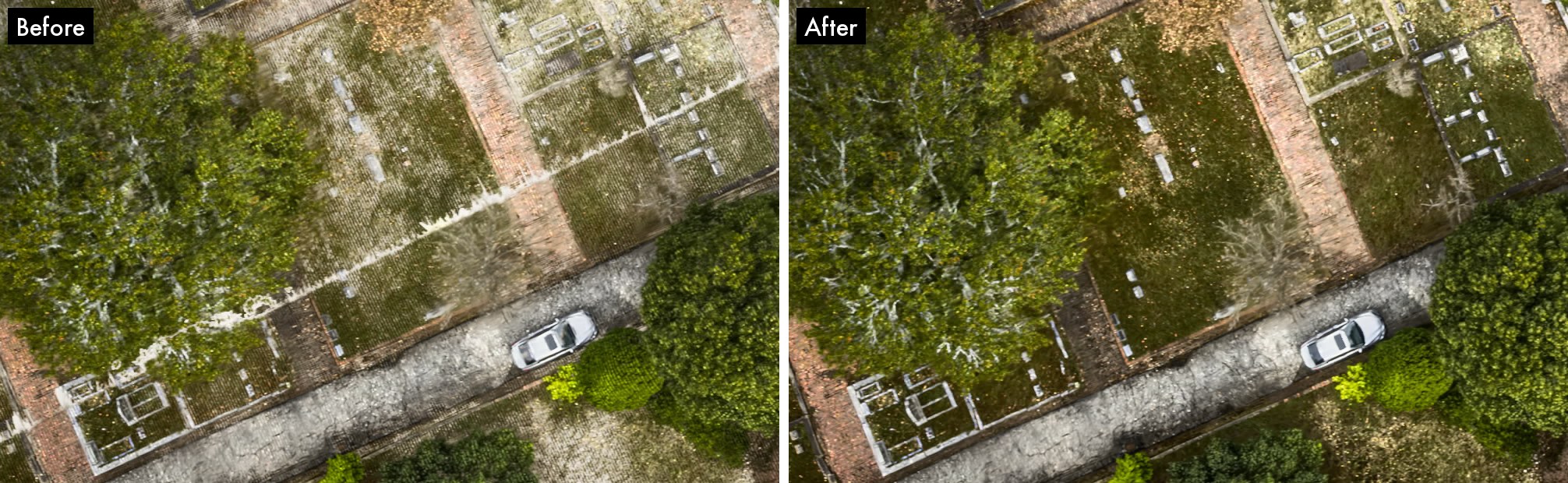
A tile seam flashing in a frame rendered with the plugin's defaults (left), and the same frame after the fix (right).

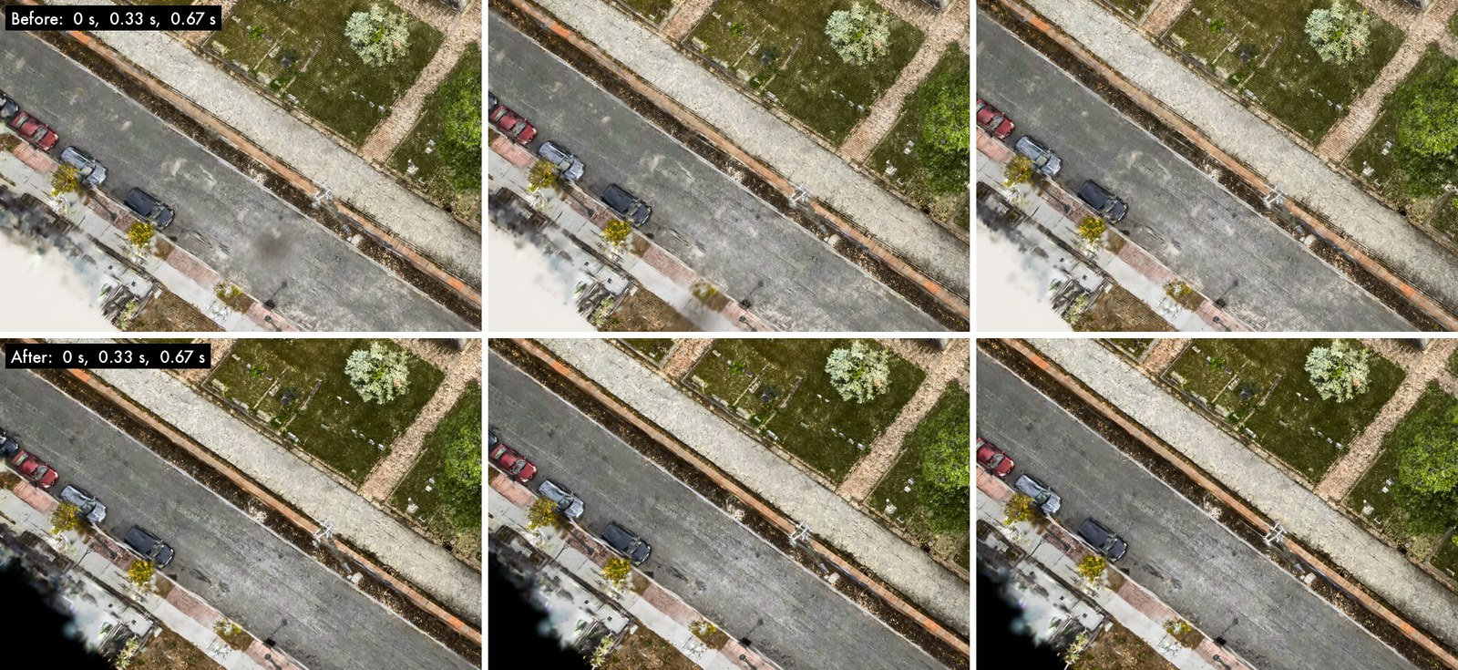
Dry road shimmering like wet pavement under the default settings, against the fixed render.

Each tile imports as its own asset at the identity transform, since the plugin converts meters and axes itself. Don't build the plugin's level-of-detail hierarchy for offline renders, or the card overflows. Every final render uses these settings, read back from the engine log afterward.

11. Check everything before publishing

Before anything is published, the engine log has to confirm the settings and the world has to match its exact gaussian count. Every frame of the film is scanned for single-frame pops, seam lines and shimmering ground, and the boundary has to come out black. Each check exists because its defect once reached a finished film.